Unsupervised learning is a type of machine learning where the user doesn’t have to watch over the model but relies on more autonomous learning. The technique enables the model to find previously unnoticed patterns and information independently. It’s primarily used where unlabeled data is unavailable or impractical. This makes it ideal for big data.
Table of Contents
If you have labelled data, read our blog post on supervised learning first.
Unlike supervised learning, unsupervised learning algorithms enable users to perform more complicated processing tasks. However, there are also some drawbacks, as the results can be more unpredictable than in other learning algorithms.

Unsupervised learning can find patterns in large data sets
Common unsupervised learning algorithms include neural networks, anomaly detection, and clustering.
Types of unsupervised learning
The three main tasks unsupervised learning models use are clustering, association, and dimensionality reduction. Dimensionality reduction is commonly used to combat the curse of dimensionality. Each learning method is defined below, with examples of common approaches and algorithms for successfully conducting them.
Clustering
In clustering, unlabeled data is grouped using data mining according to its similarities or differences. These algorithms group raw, unclassified data objects into groups that can be visualised as patterns or structures in the data. There are several clustering algorithms: exclusive or overlapping, hierarchical, and probabilistic.
Exclusive or Overlapping Clustering
A data point may only be included in one cluster in exclusive clustering or “hard” clustering. The K-means algorithm can exemplify exclusive clustering.
- K-means clustering. Data points are divided into K groups using the K-means clustering technique, which determines the number of clusters based on the distance from the centroid of each group. The data points that fall into the same category are those closest to a given centroid. Smaller K values indicate larger groupings and less granularity, while larger K values indicate smaller batches and more granularity. Market segmentation, document clustering, image segmentation, and image compression frequently use K-means clustering.
If data points can be members of multiple clusters with varying degrees of membership, we refer to these as “overlapping clusters.” Overlapping clustering is demonstrated by “soft” or fuzzy k-means clustering. This technique is commonly used in image processing. An image, for example, could contain a dog and a cat and, therefore, wouldn’t necessarily fit into just one cluster.
Hierarchical clustering
An unsupervised clustering algorithm known as hierarchical clustering, also called hierarchical cluster analysis (HCA), can be classified as either agglomerative or divisive.
The data points for agglomerative clustering are initially isolated as distinct groups and then merged iteratively based on similarity until one or more clusters are formed.
The most popular metric for calculating these distances is the Euclidean distance, but the clustering literature also mentions other metrics like the Manhattan distance.
The opposite of agglomerative clustering, divisive clustering, operates from the top down. In this instance, divisions between data points within a single data cluster are made. Even though divisive clustering is not frequently employed, it is essential to be aware of it in the context of hierarchical clustering. The merging or splitting of data points at each iteration is shown in a dendrogram; a tree-like diagram is typically used to visualise these clustering processes.
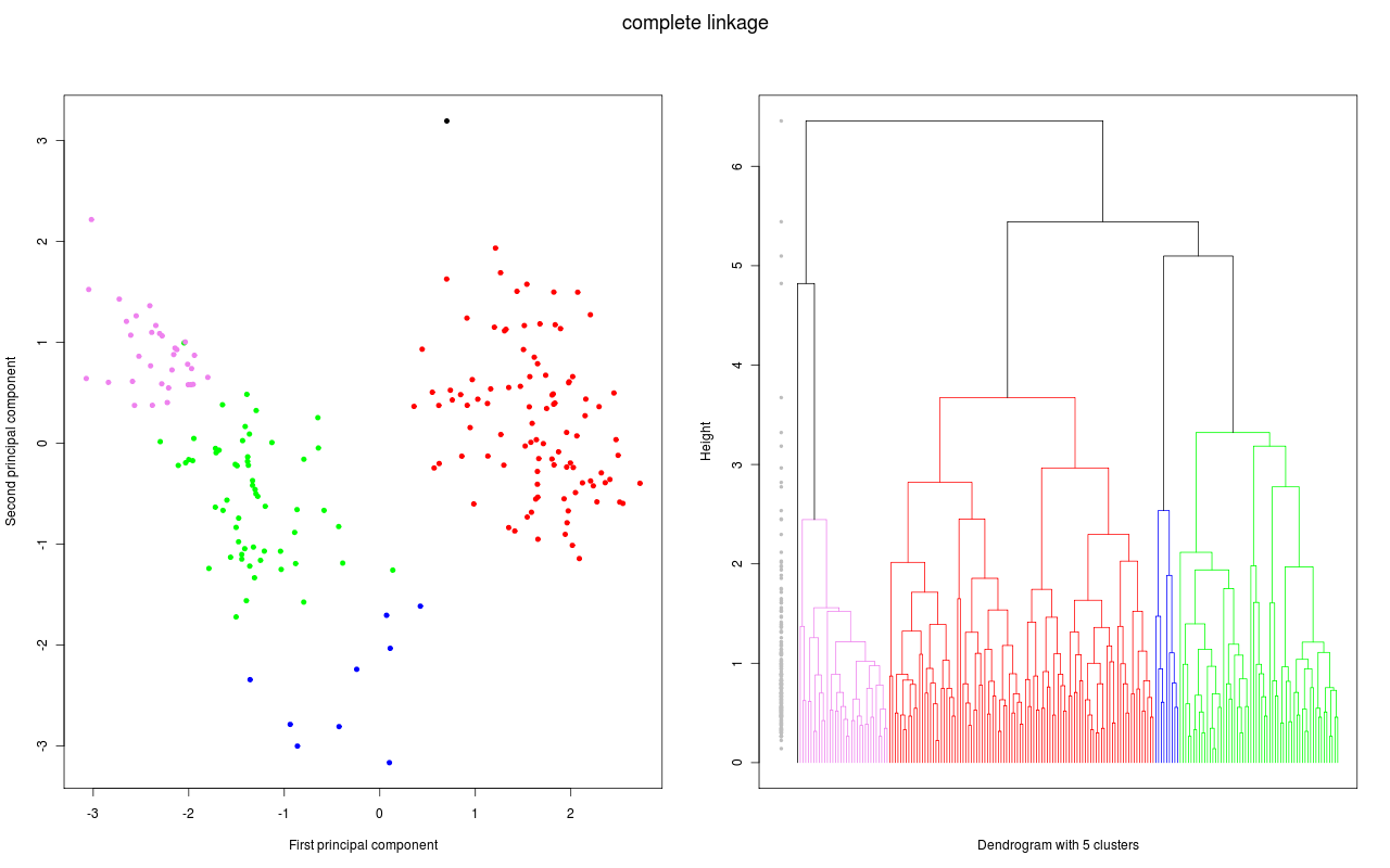
PCA vs a dendrogram
Probabilistic clustering
An unsupervised method known as a probabilistic model aids in resolving density estimation or “soft” clustering issues. Data points are grouped into probabilistic clusters according to how likely they fall under a particular distribution.
The Gaussian Mixture Model (GMM), one of the most popular probabilistic clustering techniques, was developed in the 1960s.
- Mixture models comprise an arbitrary number of probability distribution functions, of which Gaussian Mixture Models (GMM) are the best known. The main application of GMMs is to identify the Gaussian or normal probability distribution to which a given data point belongs. We can determine to which distribution a given data point belongs if the mean or variance is known. Since these variables are unknown in GMMs, we assume that a latent variable—also known as a hidden variable—exists to cluster data points appropriately. The Expectation-Maximization (EM) algorithm is frequently used to estimate the assignment probabilities for a given data point to a specific data cluster, though it is not required.
Association Rules
An association rule is a rule-based approach for identifying connections between variables in a given dataset. Market basket analysis frequently employs these techniques, which help businesses comprehend the relationships between various products. As a result, companies can create more effective cross-selling techniques and recommendation engines by better understanding consumer consumption patterns.
Apriori algorithms
Market basket analyses have made apriori algorithms more well-known, resulting in various recommendation engines for music streaming services and online shops. For example, the likelihood of consuming a product given the consumption of another product is determined by using them to identify frequent itemsets, or collections of items, within transactional datasets. This is based on prior listening habits as well as the listening habits of others.
Apriori algorithms use a hash tree to count itemsets while they traverse the dataset breadth-first.
Dimensionality reduction
More data generally produces more accurate results, but it can also affect how machine learning algorithms perform (for example, overfitting) and make it challenging to visualise datasets. A dimensionality reduction technique is used when a dataset has an excessive number of features or dimensions.
A dimensionality reduction technique keeps the dataset’s integrity as much as possible while reducing the number of data inputs to a manageable level. Several different dimensionality reduction techniques can be used:
Principal component analysis
Principal component analysis (PCA) is a type of dimensionality reduction algorithm that utilises feature extraction to reduce duplication and compress datasets. The first principal component, which is the direction that maximises the variance of the dataset, is produced by this method, which applies a linear transformation to create a new data representation, leading to a set of “principal components”.
The second principal component also finds the maximum variance in the data. Still, it is entirely unrelated to the first principal component and produces an orthogonal or perpendicular direction to the first component. Depending on the number of dimensions, this process is repeated. Each subsequent principal component points opposite from the previous component with the highest variance.
Singular value decomposition
Another dimensionality reduction technique is singular value decomposition (SVD), which factors a matrix A into three low-rank matrices. A = USVT, where U and V are orthogonal matrices, stands for SVD. The values of S, a diagonal matrix, are considered singular values of matrix A. It is frequently used to reduce noise and compress data, including image files, similar to PCA.
Autoencoders
Autoencoders use neural networks to compress data before recreating an updated version of the input from the original data. The hidden layer specifically serves as a bottleneck to compress the input layer before reconstructing it within the output layer. Encoding refers to the stage from the input layer to the hidden layer, and decoding refers to the location from the hidden layer to the output layer.
Dimensionality reduction is frequently used in the preprocessing stage.
How we use unsupervised learning
Natural language processing (NLP) lends itself well to unsupervised learning techniques. What we try to achieve is generally more complicated than predicting a single output variable. When you start working with a new data set in textual format, you must understand the documents before you. This can be done with machine learning techniques, like clustering or word cloud formation. Grouping similar documents together lets you see what the dataset comprises and how frequently abnormalities occur.

NLP is well suited to finding information in large piles of documents
Once we have a general idea of the data, we often move on to a specific task. Depending on the job, we often transform words, phrases, or sentences into vectors using word embedding or sentence embedding. These word/sentence vectors allow us to use unsupervised machine learning models that reason with the text and understand the context. This allows us to find relevant bits of information automatically within large corpora.
Knowledge graphs
Another excellent example of how we can use NLP unsupervised is creating a knowledge graph. Bits of text can be connected graphically. Graphical representation allows a user to ask natural questions and naturally open up a complicated dataset to an entire organisation. Think of this like Siri answering your questions with information from the internet. A custom-made knowledge graph can aggregate a whole organisation’s knowledge base and make it worthwhile to everyone. Future data-driven companies must rely heavily on an NLP system to remain competitive.
To conclude, even though supervised machine learning techniques are more commonly used than unsupervised machine learning techniques, there is far more potential when using unsupervised techniques. The obvious drawback is, however, that it takes more skills and resources to develop, deploy, and maintain these solutions.
Are you interested in more examples of unsupervised learning? Then, read the article on self-learning AI.
How do you use unsupervised learning? Or do you see the potential for it to be used in the future? Let us know in the comments!


0 Comments