Introduction: The Magic of Approximation
Have you ever wondered how your calculator instantly knows the value of sin(30°), e², or ln(5)? Behind that apparent magic lies a mathematical masterpiece known as the Taylor Series. This tool allows us to approximate even the most complex functions using nothing more than simple polynomials.
Table of Contents
In mathematics, approximation is a powerful idea. Most real-world problems — from predicting planetary motion to modelling stock markets or simulating physical systems — involve equations too complicated to solve exactly. Yet, we can often get incredibly close to the actual answer using a clever approximation. This is where the Taylor Series shines: it takes a smooth curve and rebuilds it piece by piece from local information — the function’s value and its derivatives at a single point.
Think of zooming in on a curve until it looks straight. At that scale, the curve behaves almost like a line — this is a first-order approximation (the tangent line). But what if you want more accuracy? Add curvature, twist, and higher-order behaviour — and suddenly, you can recreate the original function’s shape almost perfectly. That’s the idea behind the Taylor Series: a polynomial that grows more accurate as you include more terms.
From powering your calculator to helping physicists model black holes and engineers simulate flight paths, the Taylor Series is more than just an abstract formula — it’s one of the most practical and beautiful tools in all of mathematics.
The Intuition Behind Taylor Series
To truly appreciate the Taylor Series, it helps to start with an intuition rather than a formula. Imagine you’re looking at a smooth curve — say, the graph of sin(x). If you zoom in close enough around a single point, the curve begins to resemble a straight line. That line, called the tangent, gives a simple linear approximation of the function near that point.

This is the essence of local approximation — using nearby information to predict the behaviour of a function. The tangent captures the slope, or rate of change, but it misses the subtleties — the bending and curving that make the function what it is. So what if we could add more detail?
That’s precisely what the Taylor Series does. It takes not just the slope (first derivative), but also the curvature (second derivative), twist (third derivative), and so on. Each derivative reveals how the function changes at a deeper level, and when we combine them, they paint an increasingly accurate picture of the function around that point.
You can think of it as reconstructing a melody by listening to its harmonics: the more harmonics you include, the richer and closer to the original it sounds. Likewise, the more terms you add in a Taylor Series, the closer your polynomial “melody” matches the true function.
For example, the function e^x can be approximated around x=0 as:

Even with just a few terms, this simple polynomial gives a surprisingly accurate estimate of e^x for small values of x.
So, the Taylor Series is like a mathematical microscope — it lets us explore how a function behaves near any chosen point by expressing it as an infinite sum of simpler pieces. Each added layer of detail brings us closer to the original curve.
The Formal Definition of Taylor Series
Now that we’ve built an intuition for how a Taylor Series works, let’s look at its precise mathematical form.
Suppose we have a smooth function f(x), one that can be differentiated as many times as we need. The Taylor Series of f(x) around a point a is given by:

Each term in this infinite sum adds another layer of accuracy to the approximation. Let’s unpack what’s going on:
- f(a) is the value of the function at the point a. It anchors the approximation.
- f′(a)(x−a) is the linear term — the slope or tangent that captures the first level of change.
- f′′(a)/2!(x−a)^2 adjusts for the curve’s bending — how fast the slope itself is changing.
- Higher derivatives (third, fourth, etc.) add even more detail, correcting for twists and subtle inflexions.
- The factorials (2!, 3!, etc.) in the denominators ensure that each term’s contribution is scaled correctly — otherwise, the higher-order terms would quickly dominate the series.
If we choose a=0, the formula simplifies beautifully to the Maclaurin Series:

This is just a special case of the Taylor Series, centred at zero, and it’s the one most often seen in textbooks.
What makes this formula so powerful is that it doesn’t just approximate — it can exactly represent many common functions if you take infinitely many terms. For instance:

The Taylor Series gives us a universal tool: by knowing a function’s behaviour at a single point (its derivatives), we can reconstruct its shape in a neighbourhood around that point.
Classic Examples of Taylor Series
To see the Taylor Series in action, let’s look at a few classic functions — the ones that show up everywhere in mathematics, physics, and engineering. You’ll notice that many of them have beautifully simple series expansions that make complex computations surprisingly manageable.
The Exponential Function e^x

The exponential function is the shining star of the Taylor Series because its derivatives are all the same:

When evaluated at x=0:

Plugging these into the Maclaurin formula gives:

Even using just a few terms, say up to x^3, gives a remarkably close approximation for small values of x.
This series is used inside calculators and computers to compute exponential and trigonometric values efficiently.
The Sine Function sin(x)

The sine function has a cyclical pattern of derivatives:

At x=0:

Plug these into the Maclaurin Series:

Notice the alternating signs and the use of only odd powers of x. This pattern gives the wave-like shape of the sine function when summed.
The Cosine Function cos(x)

Cosine is closely related to sine, but its series starts differently:

Here, only even powers of x appear, and again, the signs alternate.
Together, the sine and cosine series describe circular motion and oscillations — the foundation of trigonometry, waves, and even quantum mechanics.
The Natural Logarithm ln(1+x)

This one behaves a bit differently because it only converges for −1<x≤1:

It’s not valid everywhere, but within its range, it provides an efficient way to estimate logarithms without a calculator.
Visualising the Series
If you plot these series — starting with a few terms, then adding more — you’ll see something fascinating.
Each partial sum approaches the actual curve of the function. For example:
- For e^x, the approximation hugs the real curve tightly near x=0 and gradually drifts for larger x.
- For sin(x), adding more terms extends the accuracy further from the origin, turning a rough line into a smooth wave.
This visual convergence shows how powerful the Taylor Series is: a simple polynomial can “learn” the shape of a complex function with stunning precision.
Convergence of Taylor Series: When Does It Work?
Up to now, the Taylor Series might seem like pure magic — turning any smooth function into an infinite polynomial.
But there’s a crucial question: does the series always work?
The answer is not always. The Taylor Series is powerful, but its success depends on how well it converges — that is, whether the infinite sum actually approaches the actual value of the function as you add more and more terms.
What Is Convergence?
A Taylor Series converges at a point x if the sum of all its terms gets closer and closer to f(x).
In mathematical terms:
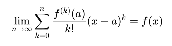
If this limit exists and equals the function’s actual value, the series converges to the function.
If it doesn’t, the approximation can drift away — sometimes dramatically.
The Radius of Convergence
Every Taylor Series has a radius of convergence, which defines how far from the centre point a the approximation remains valid.
Within that radius, the series behaves beautifully; beyond it, the approximation may break down.
For example:
- For e^x, the radius of convergence is infinite — it works everywhere.
- For sin(x) and cos(x), it’s also infinite.
- But for ln(1+x), the series only converges for −1<x≤1.
Outside that interval, the series diverges — it doesn’t represent the function at all.
The Remainder Term and Error Bound
When we use only a few terms of the Taylor Series (a truncated series), we’re making an approximation.
The difference between the actual value and our polynomial approximation is called the remainder, often written as Rn(x).
A common expression for the remainder (from the Lagrange form) is:

for some value c between a and x.
This formula tells us how much “error” we’re making by stopping at the nth term.
The smaller (x−a) and the larger n, the smaller the remainder — meaning the approximation becomes more accurate.
When Things Go Wrong
Sometimes, even though all the derivatives exist, the series fails to converge to the original function.
For instance, the function

is infinitely differentiable at x=0, but its Taylor Series around that point equals 0 for all x.
The series converges perfectly — but to the wrong function!
This reminds us that convergence alone isn’t enough; the series must also converge to the correct value.
The Beauty of Controlled Approximation
In practical terms, we rarely need an infinite number of terms.
Engineers, physicists, and computer scientists usually take just a few, enough to reach the desired accuracy.
The Taylor Series’ greatest strength lies in this balance: it lets us control how close our approximation is by deciding how many terms to keep.
Real-World Applications of Taylor Series
The Taylor Series might seem like a purely mathematical concept, but it quietly powers much of modern science, engineering, and technology. From flight simulations to smartphone chips, its ability to approximate complex functions makes it a foundational tool across disciplines. Let’s explore how it shows up in the real world.
Engineering and Physics: Modelling the Real World
In physics and engineering, most natural phenomena are governed by difficult equations—or even impossible —to solve exactly. The Taylor Series provides a way to linearise or approximate these equations so we can analyse them with manageable math.
Small-angle approximations: When modelling pendulums, waves, or vibrations, the sine function often appears. For small angles (in radians), we can use

This simple replacement allows complex motion equations to be solved analytically or simulated efficiently.
Aerodynamics and fluid dynamics: Engineers use Taylor expansions to simplify nonlinear equations describing airflow around wings or turbulence in pipes.
Relativity and quantum mechanics: Physicists often expand functions like \sqrt{1 – v^2/c^2} or wave functions into Taylor Series to analyse high-speed motion or potential energy changes.
Computer Science: Inside Your Calculator and Code
Whenever a computer or calculator computes functions like e^x sin(x), or ln(x), it’s not “looking them up” — it’s approximating them.
The underlying algorithms use truncated Taylor (or related) series to compute values with high precision quickly.
For example:
- The CORDIC algorithm, used in microprocessors and calculators, relies on series expansions to compute trigonometric and exponential functions.
- Graphics and simulations use Taylor approximations to model smooth motion, curves, and lighting changes without needing heavy computations.
Even machine learning algorithms sometimes rely on these ideas — gradient-based methods, for instance, use local linear approximations (a first-order Taylor expansion) to optimise complex functions.

Economics and Finance: Approximating Risk and Return
In economics and finance, many models describe changes in prices, interest rates, or investment returns through nonlinear functions.
Taylor expansions allow analysts to approximate these functions around a steady point, making them easier to understand and compute.
For example:
- Option pricing models (like the Black-Scholes equation) often use series expansions to approximate exponential growth or decay in asset prices.
- Elasticity analysis in economics uses first- and second-order derivatives to estimate how sensitive demand or supply is to changes in price — essentially a Taylor-series-based analysis of behaviour near a reference point.
Medicine and Biology: Modelling Living Systems
Biological systems are notoriously complex. When scientists model heartbeats, neural firing, or the spread of diseases, they often deal with nonlinear equations.
Taylor Series help them simplify these models into locally linear or quadratic approximations, which are easier to simulate and understand.
For instance:
- In neuroscience, membrane voltage equations are linearised around a resting potential using Taylor expansions.
- In epidemiology, small perturbations in infection models (e.g., SIR) are analysed using first-order approximations to predict early growth or decay trends.
Everyday Life: From GPS to Music Synthesis
Even in everyday technology, Taylor Series play a subtle role:
- GPS devices rely on approximations of the equations of satellite motion.
- Digital audio synthesis uses sine and cosine expansions to generate or process sound waves.
- Smartphone motion sensors (accelerometers and gyroscopes) use polynomial approximations to interpret data smoothly.
Common Pitfalls and Insights of Taylor Series
The Taylor Series is elegant and powerful — but it’s also easy to misuse or misunderstand. Even seasoned students and professionals sometimes stumble over a few recurring issues. Let’s unpack the most common pitfalls and the insights that help avoid them.
Confusing Convergence with Accuracy
Just because a Taylor Series converges doesn’t mean it gives a good approximation everywhere.
For example, the Taylor Series for ln(1+x) converges for −1<x≤1, but as you approach x=1, it converges very slowly. You might need dozens of terms to get a result close to the real value.
In contrast, functions like e^x converge quickly even with just a few terms.
Insight:
Always check how fast the series converges and where it converges, not just whether it does.
Forgetting the Expansion Point a
The choice of a (the point around which you expand) is crucial.
A Taylor Series is local — it’s accurate near a, but the farther you move away, the less reliable it becomes.
For instance, the series for sin(x) centered at x=0 works beautifully near zero but performs poorly near x=10π. If you need accuracy there, you’d better expand around that new point.
Insight:
The Taylor Series is not one-size-fits-all. Always choose your expansion point close to where you need accuracy.
Truncating Without Checking the Error
In practice, we can’t use an infinite number of terms — we must truncate the series.
But dropping higher-order terms without estimating the remainder can lead to significant inaccuracies.
For example, using e^x≈1+x+(x^2)/2 is fine for small x, but at x=3, it gives 8.5 instead of the true value 20.09.
The missing terms make a huge difference.
Insight:
Always estimate the remainder (the error term) to know how much trust you can place in your approximation.
Assuming Every Function Has a Useful Taylor Series
Some functions are infinitely differentiable yet have Taylor Series that fail to represent them accurately.
For example:

All derivatives at x=0 are zero, so the Taylor Series is 0 everywhere — but the actual function isn’t.
It’s a smooth curve that “escapes” its own Taylor expansion.
Insight:
Smoothness (infinitely many derivatives) doesn’t guarantee that a Taylor Series captures the true shape of a function.
Ignoring the Practical Purpose
The Taylor Series isn’t about perfection — it’s about useful approximation.
Physicists, engineers, and programmers rarely need all the terms; they care about what’s “good enough” for their purpose.
For instance, a physicist modelling small oscillations might only use the first two or three terms of sin(x). Adding more wouldn’t meaningfully improve the model — but it would unnecessarily complicate it.
Insight:
Mathematics is a tool for understanding, not just precision. The art lies in knowing when to stop.
Bonus Insight: Seeing Patterns
Once you get comfortable with Taylor Series, you start noticing patterns:
- Odd functions (like sin(x)) have only odd powers.
- Even functions (like cos(x)) have only even powers.
- Alternating signs often appear when the function oscillates.
Recognising these patterns helps you predict a function’s behaviour without even computing all its derivatives.
Conclusion: Why Taylor Series Matter
The Taylor Series is more than just another formula in the calculus toolbox — it’s a bridge between the ideal and the real, between pure math and practical application. It shows us that even the most complex, wavy, or nonlinear function can be understood as a sum of simple, familiar pieces: powers of x.
At its heart, the Taylor Series represents one of the deepest ideas in mathematics — that local information can reveal global behaviour. By knowing how a function behaves at a single point (its derivatives), we can reconstruct its curve, predict its values, and even model entire physical systems.
This principle is everywhere:
- Physicists use it to predict motion under the influence of gravity.
- Engineers use it to simulate how structures bend or oscillate.
- Computer scientists use it to efficiently approximate exponential and trigonometric functions.
- Economists and biologists use it to model changes and growth around stable states.
It’s a quiet hero of modern computation — silently powering everything from GPS navigation to AI optimisation algorithms.
But beyond its utility, there’s a certain elegance to it. The Taylor Series captures the essence of approximation — the idea that perfection is often unnecessary, and that progress comes from refining small steps. With each added term, you get closer to the truth, and that mirrors how understanding itself works: incrementally, patiently, beautifully.
Or, as mathematician Henri Poincaré once said:
“Mathematics is the art of giving the same name to different things.”
The Taylor Series is a perfect example — the same simple polynomial can become a sine wave, an exponential, or a logarithm, depending on how we shape it.


0 Comments