What is Dynamic Programming?
Dynamic Programming (DP) is a powerful algorithmic technique used to solve complex problems by breaking them down into simpler, overlapping subproblems. Instead of solving the same subproblem multiple times, DP solves each subproblem once, stores the result, and reuses it when needed. This approach often turns exponential-time algorithms into efficient polynomial-time solutions.
Table of Contents
Two key principles make DP possible:
- Optimal Substructure: A problem exhibits optimal substructure if the optimal solution to the overall problem can be constructed from the optimal solutions of its subproblems. For example, the shortest path between two cities can be found by combining the shortest paths of intermediate segments.
- Overlapping Subproblems: Many problems, especially recursive ones, solve the same subproblems multiple times. DP takes advantage of this by storing the results (memoisation) or computing them in a systematic order (tabulation), avoiding redundant work.
Difference from Divide and Conquer:
While Divide and Conquer also breaks a problem into subproblems, these subproblems are usually independent. In contrast, DP works best when subproblems overlap and their results can be reused.
Example:
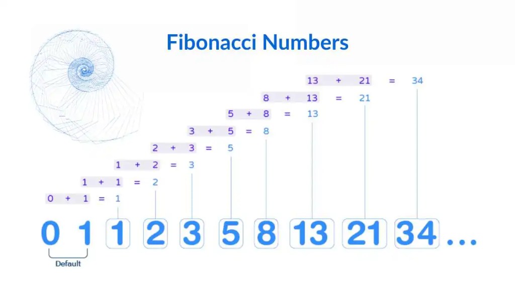
Calculating the nth Fibonacci number recursively involves repeated calculations of the same numbers. Using DP, each Fibonacci number is computed only once and stored, drastically improving efficiency.
Dynamic Programming is widely used in optimisation, pathfinding, scheduling, and even AI, making it an essential tool for any programmer or algorithm enthusiast.
Real-World Examples of Dynamic Programming Problems
Dynamic Programming isn’t just a theoretical concept—it powers many real-world applications where efficiency and optimal decisions matter. Here are some examples:
1. Shortest Path in Maps
Navigation systems rely on DP to find the most efficient route. Algorithms like Bellman-Ford or Floyd-Warshall use DP to compute shortest paths between cities or nodes in a network, taking into account distances, traffic, or other constraints.
2. Text Processing and Spell Checking
Applications like autocorrect, text search, and plagiarism detection use DP. For instance, the Edit Distance problem calculates the minimum number of insertions, deletions, or substitutions needed to convert one string into another. DP efficiently computes this for large texts.
3. Game Theory & AI Decision-Making
DP helps AI plan optimal strategies in games. For example, in chess or tic-tac-toe, DP can evaluate game states and decide the best moves, storing results of previously analysed positions to avoid redundant calculations.
4. Financial Planning & Optimisation
Problems like maximising profit from stock trades, budgeting, or resource allocation can be solved using DP. Algorithms like the Knapsack Problem determine the best combination of investments or resources under constraints to achieve optimal outcomes.
5. Scheduling & Resource Allocation
DP is used in job scheduling, project planning, and network bandwidth allocation. It helps optimise for minimum completion time, maximum efficiency, or balanced workloads, even when tasks have dependencies or limited resources.
6. Bioinformatics
DP is crucial in DNA sequence alignment, protein folding, and other computational biology tasks. For example, the Needleman-Wunsch and Smith-Waterman algorithms align genetic sequences efficiently to find similarities and differences.
Whenever a problem involves making a sequence of decisions to optimise a goal, and overlapping subproblems appear, DP is often the ideal approach. It transforms problems that would be infeasible to solve with brute force into efficient, practical solutions.
Two Core Approaches to Dynamic Programming in Python
Dynamic Programming problems can generally be solved using two main approaches: Top-Down (Memoisation) and Bottom-Up (Tabulation). Both aim to avoid redundant calculations, but they differ in execution and structure.
1. Top-Down Approach (Memoisation)
Concept: Start with the original problem and break it into smaller subproblems recursively. Store the results of subproblems in a cache or dictionary so they are not recomputed.
How it works:
- Check if the result for the current subproblem is already computed.
- If yes, return the cached result.
- If no, compute it recursively and store the result.
Pros: Intuitive and easy to implement if you already know the recursive solution.
Cons: Can have extra overhead due to the recursion stack.
Example: Fibonacci numbers (Top-Down)
def fib(n, memo={}):
if n in memo:
return memo[n]
if n <= 1:
return n
memo[n] = fib(n-1, memo) + fib(n-2, memo)
return memo[n]
print(fib(10)) # Output: 552. Bottom-Up Approach (Tabulation)
Concept: Solve all smaller subproblems first, then combine them to solve larger subproblems. Usually implemented iteratively using a table (array).
How it works:
- Define a table to store the results of subproblems.
- Fill the table in a logical order so that when you compute a subproblem, all smaller subproblems it depends on are already solved.
Pros: Avoids recursion and stack overflow; can be more memory-efficient.
Cons: Requires identifying the correct order to fill the table.
Example: Fibonacci numbers (Bottom-Up)
def fib(n):
if n <= 1:
return n
dp = [0] * (n+1)
dp[1] = 1
for i in range(2, n+1):
dp[i] = dp[i-1] + dp[i-2]
return dp[n]
print(fib(10)) # Output: 55When to Use Which Approach
Use Top-Down if the problem is naturally recursive and you want simplicity.
Use Bottom-Up if recursion depth is a concern or for more predictable performance.
Key Idea: Both approaches achieve the same goal: compute each subproblem only once. The choice is mainly about readability and performance constraints.
Step-by-Step Method for Solving a Dynamic Programming Problem
Solving a Dynamic Programming problem can seem tricky at first, but following a systematic approach can make it manageable. Here’s a step-by-step framework you can use for almost any DP problem:
Step 1: Identify Overlapping Subproblems
Look for problems where the same calculations are repeated multiple times.
Examples: Fibonacci numbers, shortest paths, knapsack.
Tip: Draw a recursion tree for the naive solution to visualise repeated subproblems.
Step 2: Check for Optimal Substructure
Determine if the solution to the overall problem can be composed from optimal solutions to smaller subproblems.
Example: The shortest path from A to C can be broken down into the shortest path from A to B plus the shortest path from B to C.
Step 3: Define the State
Decide what parameters uniquely identify each subproblem.
The state is usually represented as a tuple of variables.
Example: For the knapsack problem, a state can be (i, w) where i is the current item index and w is the remaining capacity.
Step 4: Write the Recurrence Relation
Express the solution of a subproblem in terms of smaller subproblems.
This forms the backbone of the DP algorithm.
Example: Fibonacci: fib(n) = fib(n-1) + fib(n-2)
Step 5: Choose Memoisation or Tabulation
Top-Down (Memoisation): Recursive approach with caching.
Bottom-Up (Tabulation): An Iterative approach using a table.
Pick based on the problem size, recursion depth, and personal preference.
Step 6: Implement the Dynamic Programming Solution
Start with a small example to test correctness.
Make sure to handle base cases properly.
Optimise space if possible (e.g., rolling arrays for 1D or 2D DP).
Step 7: Test and Optimise
Check against known results or edge cases.
Analyse time and space complexity.
Consider reducing memory usage or simplifying the state if needed.
Example in Practice: Climbing Stairs
- Problem: You can climb 1 or 2 steps at a time. How many ways are there to reach step n?
- State: dp[i] = ways to reach step i
- Recurrence: dp[i] = dp[i-1] + dp[i-2]
- Base cases: dp[0] = 1, dp[1] = 1
- Solution (Bottom-Up):
def climb_stairs(n):
if n <= 1:
return 1
dp = [0] * (n+1)
dp[0], dp[1] = 1, 1
for i in range(2, n+1):
dp[i] = dp[i-1] + dp[i-2]
return dp[n]
print(climb_stairs(5)) # Output: 8Classic Dynamic Programming Problems and Their Patterns
Dynamic Programming problems often follow common patterns. Recognising these patterns makes it much easier to approach new problems. Here are some of the most common DP problem types:
1. 1D Dynamic Programming (Linear Dynamic Programming)
Pattern: Solve problems over a single dimension like time, steps, or items.
Typical Problems:
- Fibonacci numbers
- Climbing stairs
- Maximum sum subarray (Kadane’s algorithm)
Key Idea: dp[i] depends only on a few previous states, e.g., dp[i-1], dp[i-2].
2. 2D Dynamic Programming (Grid/Matrix Dynamic Programming)
Pattern: Solve problems over a two-dimensional grid or matrix.
Typical Problems:
- Knapsack problem
- Minimum path sum in a grid
- Longest common subsequence (LCS)
Key Idea: dp[i][j] represents the solution for the first i elements of one sequence and the first j elements of another, or the first i rows and j columns of a grid.
3. Interval Dynamic Programming
Pattern: Solve problems on subarrays or intervals where the solution depends on splitting an interval into smaller intervals.
Typical Problems:
- Matrix chain multiplication
- Burst balloons problem
- Optimal game strategies
Key Idea: dp[i][j] represents the solution for the interval from i to j.
4. Bitmask Dynamic Programming
Pattern: Solve problems over subsets using a bitmask to represent selected elements.
Typical Problems:
- Travelling Salesman Problem (TSP)
- Subset sum
- Assignment problems
Key Idea: dp[mask][i] represents the best solution for a subset mask ending at element i.
5. State Machine Dynamic Programming
Pattern: Solve problems that involve states changing over time, often with constraints.
Typical Problems:
- Stock buy/sell with cooldown.
- Robot movement with conditions
- Weather simulation problems
Key Idea: Each state encodes enough information to represent the current condition and make decisions.
Once you learn to identify the DP pattern, solving a new problem becomes easier. Most DP problems are variations or combinations of these patterns. Start by asking:
- Is it linear, 2D, interval, subset, or state-based?
- What is the state representation?
- What is the recurrence relation?
Common Pitfalls and How to Avoid Them
Dynamic Programming can be tricky, especially for beginners. Here are some common mistakes and tips on how to avoid them:
1. Not Identifying Overlapping Subproblems
Pitfall: Treating every subproblem as unique and recalculating it repeatedly, leading to slow, exponential-time solutions.
How to Avoid: Draw a recursion tree for the naive solution to see which subproblems repeat. Use memoisation or tabulation to store and reuse results.
2. Incorrect State Definition
Pitfall: Choosing the wrong parameters for your DP state, which can make it impossible to write a correct recurrence relation.
How to Avoid: Clearly define what each subproblem represents and ensure it uniquely identifies the computation needed. Test small examples to confirm.
3. Forgetting Base Cases
Pitfall: Not initialising base cases or handling edge cases, leading to incorrect or undefined results.
How to Avoid: Identify the simplest subproblems (usually size 0 or 1) and explicitly define their results before building larger solutions.
4. Ignoring Memory Optimisation
Pitfall: Using a full DP table even when only a few previous states are needed, wasting memory.
How to Avoid: Use rolling arrays or reduce dimensions when possible. For example, Fibonacci numbers need only the last two results instead of the entire array.
5. Confusing Recursion vs. Iteration
Pitfall: Mixing top-down and bottom-up approaches incorrectly, leading to redundant calculations or stack overflows.
How to Avoid: Stick to one approach per problem. Use memoisation for recursive clarity, or tabulation for iterative efficiency.
6. Overcomplicating the Problem
Pitfall: Trying to solve the entire problem at once without breaking it into subproblems.
How to Avoid: Start small. Solve a smaller instance first, understand its pattern, and then generalise to the whole problem.
7. Not Analysing Complexity
Pitfall: Assuming a DP solution is always fast; some DP states can grow exponentially if not carefully defined.
How to Avoid: Count the number of unique states and the work per state—Optimise state representation to reduce time and space complexity.
Performance Considerations
Dynamic Programming is powerful, but it can also be resource-intensive if not carefully designed. Understanding performance considerations helps you write efficient DP solutions.
1. Time Complexity
Definition: Time complexity depends on the number of unique subproblems and the time spent per subproblem.
How to Analyse:
- Count the number of possible states (size of your DP table).
- Multiply by the time required to compute each state.
Example:
- Fibonacci DP: O(n) states × O(1) computation = O(n)
- 0/1 Knapsack DP: O(n*W) states × O(1) computation = O(n*W)
2. Space Complexity
Issue: Storing large DP tables can consume a lot of memory.
Optimisation Techniques:
- Rolling Arrays: Store only the last few relevant states instead of the entire table.
- State Compression: Use bitmasks or reduced dimensions when possible.
Example: Fibonacci numbers can be computed using two variables instead of an array of size n.
3. Choosing the Right Approach
Top-Down (Memoisation):
- Pros: Easier to implement for complex recursive problems.
- Cons: Extra recursion stack space; may be slower due to function call overhead.
Bottom-Up (Tabulation):
- Pros: Iterative, predictable memory usage, no recursion overhead.
- Cons: May require careful ordering of subproblems.
4. Avoiding Redundant Computations
- Ensure each subproblem is computed only once.
- Use memoisation tables or DP arrays correctly.
- Avoid unnecessary loops or recomputation inside DP state updates.
5. Special Cases and Trade-offs
Sometimes a simpler algorithm may outperform DP for small inputs.
Consider hybrid approaches:
- Combine DP with greedy methods for partial optimisation.
- Use pruning techniques in recursive DP to skip irrelevant states.
Efficient DP is about balancing time and space. Analyse the number of states, work per state, and memory usage. Optimising these factors ensures your solution runs fast and scales well for larger inputs.
Dynamic Programming in Practice
Dynamic Programming is more than just an academic concept—it’s widely used in real-world applications across software development, data science, and optimisation problems. Understanding how DP works in practice helps you apply it effectively.
1. Software Development and Algorithms
DP is often used to solve classic algorithmic challenges in coding interviews and competitive programming.
Examples:
- Pathfinding: Shortest path in a grid or weighted graph.
- String Matching: Longest Common Subsequence (LCS), edit distance.
- Resource Allocation: Knapsack problem, job scheduling.
2. Data Science and Machine Learning
DP can optimise computationally heavy tasks by caching intermediate results.
Examples:
- Sequence Modelling: Dynamic programming underpins some algorithms in bioinformatics (DNA sequence alignment).
- Probabilistic Models: Hidden Markov Models (HMMs) use DP for efficient likelihood calculations.
3. Operations Research and Optimisation
Many optimisation problems in logistics, finance, and planning are solved using DP.
Examples:
- Inventory Management: Minimising costs over time with stock constraints.
- Portfolio Optimisation: Choosing optimal investments across multiple periods.
- Resource Scheduling: Assigning tasks efficiently under constraints.
4. Game Development
DP can help compute optimal strategies or simulate outcomes in games.
Examples:
- Turn-based strategy games (optimal moves).
- AI for board games like chess or checkers (minimax with DP memoisation).
5. Key Practices for Using DP in Real Projects
- Start Simple: Solve a miniature version of the problem first.
- Profile Your Solution: Identify bottlenecks in time or memory.
- Use Efficient Data Structures: Hash maps, arrays, or bitmasks, depending on the state representation.
- Combine Techniques: Sometimes DP works best with greedy, divide-and-conquer, or graph algorithms.
Dynamic Programming is a practical and versatile tool. By understanding patterns, optimising performance, and recognising real-world applications, you can tackle complex problems efficiently—whether in coding challenges, research, or software projects.
Conclusion
Dynamic Programming (DP) is one of the most potent techniques in problem-solving, allowing you to tackle complex problems by breaking them into manageable subproblems. From algorithmic challenges to real-world applications in software development, data science, and optimisation, DP provides a structured way to achieve efficient solutions.
Key Takeaways:
- Identify Overlapping Subproblems: Recognise repeated calculations to avoid redundant work.
- Understand Optimal Substructure: Ensure the problem can be built from smaller, optimal solutions.
- Choose the Right Approach: Decide between top-down (memoisation) and bottom-up (tabulation) based on the problem and resources.
- Optimise Time and Space: Carefully design states and recurrence relations to balance performance.
- Learn Common Patterns: 1D, 2D, interval, bitmask, and state machine DP patterns help solve new problems faster.
- Avoid Pitfalls: Define states correctly, handle base cases, and prevent unnecessary recomputation.
- Apply DP in Practice: DP is not just academic—it powers real-world applications like pathfinding, scheduling, sequence analysis, and AI strategy.
Mastering DP takes practice, patience, and pattern recognition. By following a structured approach and analysing performance, you can confidently tackle problems that might initially seem overwhelming. Remember: every DP problem is just a combination of smaller, solvable pieces—once you see the pieces, the solution becomes clear.


0 Comments